Background: Understanding Learned Optimizers
What are Learned Optimizers?
Traditional optimization algorithms like Adam, SGD, and Adafactor rely on hand-designed update rules that have been carefully crafted by researchers over decades. While these optimizers work well across many tasks, they come with limitations:
They require careful hyperparameter tuning (learning rate, momentum, weight decay)
They use the same update rule for all parameters and all tasks
Learned optimizers take a different approach: they use machine learning to discover optimization algorithms. Instead of hand-designing update rules, we train a small neural network (the “learned optimizer”) to predict good parameter updates based on the training history.
The key insight is that optimization itself is a learnable problem. By training an optimizer on thousands of different tasks, it can learn patterns about how to efficiently navigate loss landscapes that generalize to new, unseen tasks.
How Do Learned Optimizers Work?
The Core Idea
At each training step, a learned optimizer processes rich information about the current state of training and predicts how to update each parameter. Let’s compare the approaches:
Traditional Optimizer (Adam):
# Simple hand-designed update rule
m = β₁ × m + (1 - β₁) × gradient        # momentum
v = β₂ × v + (1 - β₂) × gradient²       # second moment
update = learning_rate × m / (√v + ε)
parameter = parameter - update
Learned Optimizer:
# Neural network predicts the update
features = construct_features(gradient, momentum, second_moment,
                               parameter, timestep, ...)
features = normalize(features)
direction, magnitude = MLP(features)
update = direction × exp(magnitude × α) × β
parameter = parameter - update
The learned optimizer’s MLP is small (typically 2-3 hidden layers with 32-64 units) but has been meta-trained on thousands of optimization tasks to make good predictions.
Feature Construction
Learned optimizers construct a rich set of features to inform their decisions:
Accumulator-based features:
Momentum accumulators (like Adam’s first moment):
m_t = β × m_{t-1} + (1-β) × ∇Second moment estimates (like Adam’s second moment):
v_t = β × v_{t-1} + (1-β) × ∇²Factored second moments (inspired by Adafactor): row and column factors for efficient memory usage
Derived features:
Normalized momentum:
m / √vReciprocal square roots:
1 / √vInteraction features: combinations of gradients with momentum and factored terms
Parameter values: the current weights being optimized
Gradient values: raw and clipped gradient information
Temporal features:
Time-based features using
tanh(t / x)for various time scalesThese help the optimizer adapt its behavior over the course of training
Note
See Appendix G of the paper for complete feature tables for VeLO and small_fc_lopt.
The Optimization Pipeline
Here’s what happens during a single optimizer step:
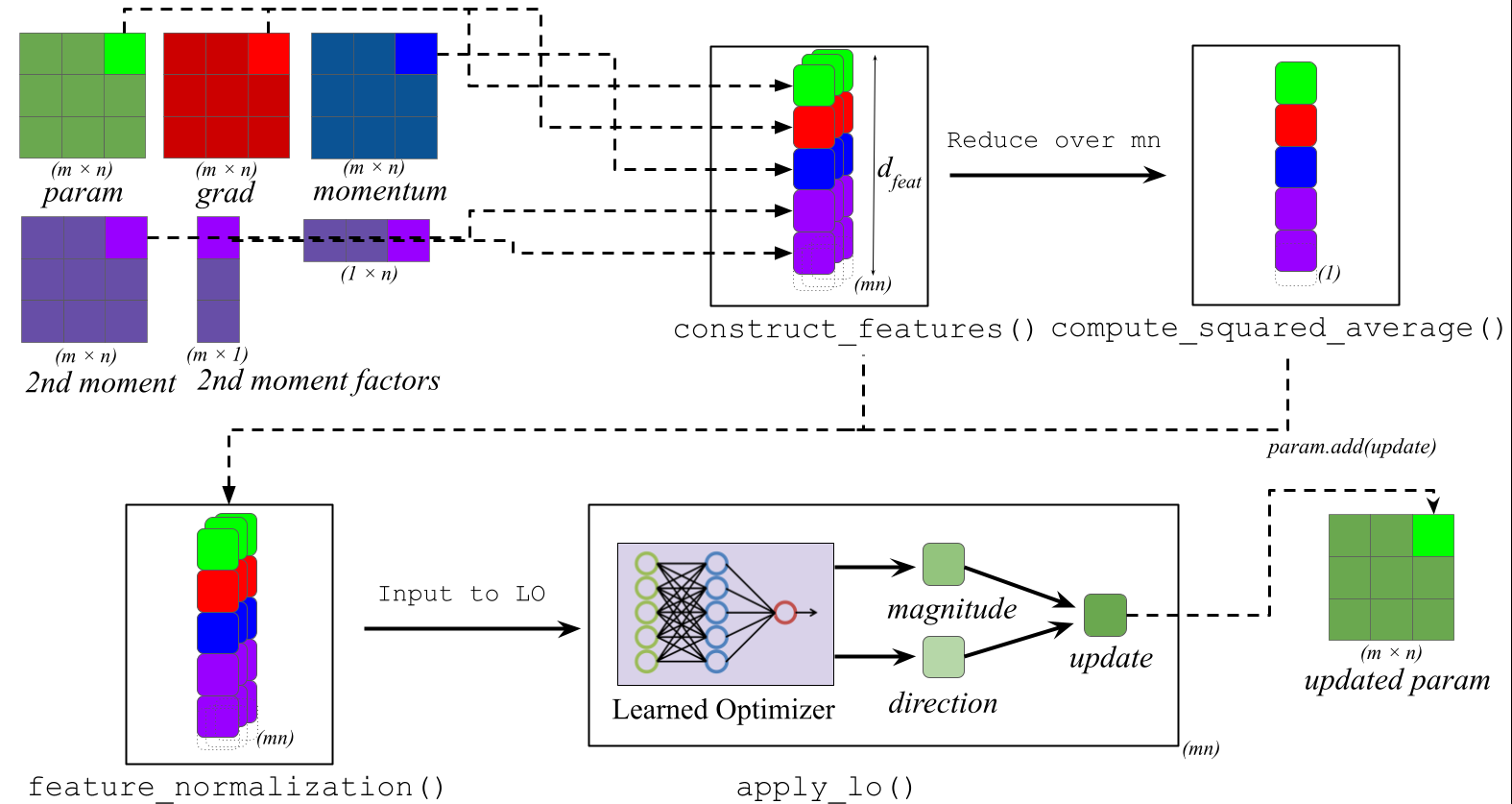
1. Update Accumulators
   ├─→ momentum: m = β₁m + (1-β₁)∇
   ├─→ second moment: v = β₂v + (1-β₂)∇²
   └─→ factored moments: r, c (row/column factors)

2. Construct Features
   ├─→ Raw values: ∇, θ, m, v, r, c
   ├─→ Combinations: m/√v, ∇·√(r⊗c), etc.
   └─→ Time features: tanh(t/1), tanh(t/10), ..., tanh(t/10⁵)

3. Normalize Features
   └─→ Divide by √(mean(feature²) + ε)

4. Apply Learned Optimizer MLP
   ├─→ hidden = ReLU(Linear1(features))
   ├─→ hidden = ReLU(Linear2(hidden))
   └─→ direction, magnitude = Linear3(hidden)

5. Compute and Apply Update
   └─→ θ ← θ - direction × exp(magnitude × α) × β
Meta-Training: How Learned Optimizers Learn
Learned optimizers are trained through a process called meta-learning:
Sample a random task (e.g., train a small CNN on CIFAR-10)
Unroll optimization for K steps using the learned optimizer
Compute meta-loss based on the final validation/ training loss
Update the optimizer’s weights via gradient estimation strategies such as Evolution Strategies.
Repeat for thousands of diverse tasks
This is computationally expensive and SOTA learned optimizer VeLO was meta-trained for 4000 TPU-months! but needs to be done only once. The resulting learned optimizer can then be applied to new tasks without retraining. Similar to how pretraining is done in LLMs.
Important
You don’t need to meta-train learned optimizers yourself. PyLO provides pre-trained optimizers ready to use. Think of it like using a pre-trained language model: the expensive training has already been done.
References and Further Reading
Key Papers:
VeLO: Training Versatile Learned Optimizers by Scaling Up (Metz et al., 2022)
The paper introducing VeLO, meta-trained for 4000 TPU-months
μLO: Compute-Efficient Meta-Generalization of Learned Optimizers (Thérien et al., 2024)
The small_fc_lopt optimizer optimized for compute efficiency using Maximum update parameterization
Celo: Training Versatile Learned Optimizers on a Compute Diet (Moudgil et al., 2025)
Introduces Celo, a learned optimizer trained on a diverse set of tasks with limited compute budget
Practical tradeoffs between memory, compute, and performance in learned optimizers (Metz et al., 2022)
The foundational paper that introduces small_fc_lopt and discusses tradeoffs in learned optimizers
Unbiased Gradient Estimation in Unrolled Computation Graphs with Persistent Evolution Strategies (Vicol et al., 2021)
The paper that introduces Persistent Evolution Strategies for meta-training learned optimizers
PyLO: Towards Accessible Learned Optimizers in PyTorch (Janson et al., 2025)
This paper! Details PyLO’s design and benchmarks
Codebases:
google/learned_optimization - Original JAX implementation
Belilovsky-Lab/pylo - This PyTorch implementation
Belilovsky-Lab/pylo-examples - Training examples